概述
本文将详细展示一个多类支持向量机分类器训练iris数据集来分类三种花。
SVM算法最初是为二值分类问题设计的,但是也可以通过一些策略使得其能进行多类分类。主要的两种策略是:一对多(one versus all)方法;一对一(one versus one)方法。
一对一方法是在任意两类样本之间设计创建一个二值分类器,然后得票最多的类别即为该未知样本的预测类别。但是当类别(k类)很多的时候,就必须创建k!/(k-2)!2!个分类器,计算的代价还是相当大的。
另外一种实现多类分类器的方法是一对多,其为每类创建一个分类器。最后的预测类别是具有最大SVM间隔的类别。本文将实现该方法。
我们将加载iris数据集,使用高斯核函数的非线性多类SVM模型。iris数据集含有三个类别,山鸢尾、变色鸢尾和维吉尼亚鸢尾(I.setosa、I.virginica和I.versicolor),我们将为它们创建三个高斯核函数SVM来预测。
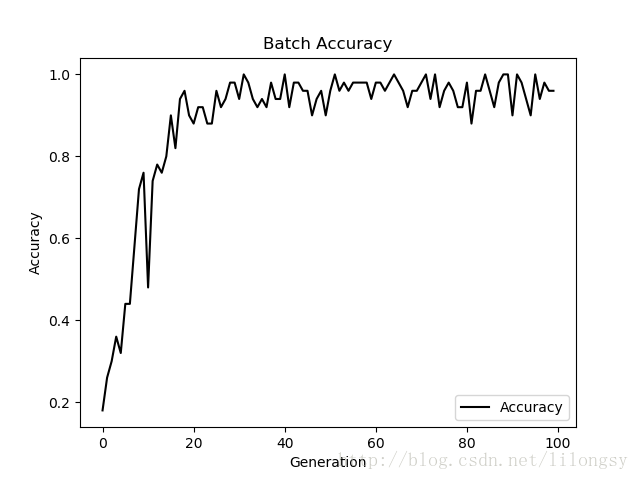
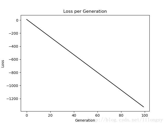
# Multi-class (Nonlinear) SVM Example
#----------------------------------
#
# This function wll illustrate how to
# implement the gaussian kernel with
# multiple classes on the iris dataset.
#
# Gaussian Kernel:
# K(x1,x2) = exp(-gamma * abs(x1 - x2)^2)
#
# X : (Sepal Length,Petal Width)
# Y: (I. setosa,I. virginica,I. versicolor) (3 classes)
#
# Basic idea: introduce an extra dimension to do
# one vs all classification.
#
# The prediction of a point will be the category with
# the largest margin or distance to boundary.

import matplotlib.pyplot as plt
import numpy as np
import tensorflow as tf
from sklearn import datasets
from tensorflow.python.framework import ops
ops.reset_default_graph()

# Create graph
sess = tf.Session()

# Load the data
# 加载iris数据集并为每类分离目标值。
# 因为我们想绘制结果图,所以只使用花萼长度和花瓣宽度两个特征。
# 为了便于绘图,也会分离x值和y值
# iris.data = [(Sepal Length,Sepal Width,Petal Length,Petal Width)]
iris = datasets.load_iris()
x_vals = np.array([[x[0],x[3]] for x in iris.data])
y_vals1 = np.array([1 if y==0 else -1 for y in iris.target])
y_vals2 = np.array([1 if y==1 else -1 for y in iris.target])
y_vals3 = np.array([1 if y==2 else -1 for y in iris.target])
y_vals = np.array([y_vals1,y_vals2,y_vals3])
class1_x = [x[0] for i,x in enumerate(x_vals) if iris.target[i]==0]
class1_y = [x[1] for i,x in enumerate(x_vals) if iris.target[i]==0]
class2_x = [x[0] for i,x in enumerate(x_vals) if iris.target[i]==1]
class2_y = [x[1] for i,x in enumerate(x_vals) if iris.target[i]==1]
class3_x = [x[0] for i,x in enumerate(x_vals) if iris.target[i]==2]
class3_y = [x[1] for i,x in enumerate(x_vals) if iris.target[i]==2]

# Declare batch size
batch_size = 50

# Initialize placeholders
# 数据集的维度在变化,从单类目标分类到三类目标分类。
# 我们将利用矩阵传播和reshape技术一次性计算所有的三类SVM。
# 注意,由于一次性计算所有分类,
# y_target占位符的维度是[3,None],模型变量b初始化大小为[3,batch_size]
x_data = tf.placeholder(shape=[None,2],dtype=tf.float32)
y_target = tf.placeholder(shape=[3,None],dtype=tf.float32)
prediction_grid = tf.placeholder(shape=[None,dtype=tf.float32)

# Create variables for svm
b = tf.Variable(tf.random_normal(shape=[3,batch_size]))

# Gaussian (RBF) kernel 核函数只依赖x_data
gamma = tf.constant(-10.0)
dist = tf.reduce_sum(tf.square(x_data),1)
dist = tf.reshape(dist,[-1,1])
sq_dists = tf.multiply(2.,tf.matmul(x_data,tf.transpose(x_data)))
my_kernel = tf.exp(tf.multiply(gamma,tf.abs(sq_dists)))

# Declare function to do reshape/batch multiplication
# 最大的变化是批量矩阵乘法。
# 最终的结果是三维矩阵,并且需要传播矩阵乘法。
# 所以数据矩阵和目标矩阵需要预处理,比如xT?x操作需额外增加一个维度。
# 这里创建一个函数来扩展矩阵维度,然后进行矩阵转置,
# 接着调用TensorFlow的tf.batch_matmul()函数
def reshape_matmul(mat):
  v1 = tf.expand_dims(mat,1)
  v2 = tf.reshape(v1,[3,batch_size,1])
  return(tf.matmul(v2,v1))

# Compute SVM Model 计算对偶损失函数
first_term = tf.reduce_sum(b)
b_vec_cross = tf.matmul(tf.transpose(b),b)
y_target_cross = reshape_matmul(y_target)

second_term = tf.reduce_sum(tf.multiply(my_kernel,tf.multiply(b_vec_cross,y_target_cross)),[1,2])
loss = tf.reduce_sum(tf.negative(tf.subtract(first_term,second_term)))

# Gaussian (RBF) prediction kernel
# 现在创建预测核函数。
# 要当心reduce_sum()函数,这里我们并不想聚合三个SVM预测,
# 所以需要通过第二个参数告诉TensorFlow求和哪几个
rA = tf.reshape(tf.reduce_sum(tf.square(x_data),1),1])
rB = tf.reshape(tf.reduce_sum(tf.square(prediction_grid),1])
pred_sq_dist = tf.add(tf.subtract(rA,tf.multiply(2.,tf.transpose(prediction_grid)))),tf.transpose(rB))
pred_kernel = tf.exp(tf.multiply(gamma,tf.abs(pred_sq_dist)))

# 实现预测核函数后,我们创建预测函数。
# 与二类不同的是,不再对模型输出进行sign()运算。
# 因为这里实现的是一对多方法,所以预测值是分类器有最大返回值的类别。
# 使用TensorFlow的内建函数argmax()来实现该功能
prediction_output = tf.matmul(tf.multiply(y_target,b),pred_kernel)
prediction = tf.arg_max(prediction_output-tf.expand_dims(tf.reduce_mean(prediction_output,0)
accuracy = tf.reduce_mean(tf.cast(tf.equal(prediction,tf.argmax(y_target,0)),tf.float32))

# Declare optimizer
my_opt = tf.train.GradientDescentOptimizer(0.01)
train_step = my_opt.minimize(loss)

# Initialize variables
init = tf.global_variables_initializer()
sess.run(init)

# Training loop
loss_vec = []
batch_accuracy = []
for i in range(100):
  rand_index = np.random.choice(len(x_vals),size=batch_size)
  rand_x = x_vals[rand_index]
  rand_y = y_vals[:,rand_index]
  sess.run(train_step,Feed_dict={x_data: rand_x,y_target: rand_y})

  temp_loss = sess.run(loss,y_target: rand_y})
  loss_vec.append(temp_loss)

  acc_temp = sess.run(accuracy,y_target: rand_y,prediction_grid:rand_x})
  batch_accuracy.append(acc_temp)

  if (i+1)%25==0:
    print('Step #' + str(i+1))
    print('Loss = ' + str(temp_loss))

# 创建数据点的预测网格,运行预测函数
x_min,x_max = x_vals[:,0].min() - 1,x_vals[:,0].max() + 1
y_min,y_max = x_vals[:,1].min() - 1,1].max() + 1
xx,yy = np.meshgrid(np.arange(x_min,x_max,0.02),np.arange(y_min,y_max,0.02))
grid_points = np.c_[xx.ravel(),yy.ravel()]
grid_predictions = sess.run(prediction,prediction_grid: grid_points})
grid_predictions = grid_predictions.reshape(xx.shape)

# Plot points and grid
plt.contourf(xx,yy,grid_predictions,cmap=plt.cm.Paired,alpha=0.8)
plt.plot(class1_x,class1_y,'ro',label='I. setosa')
plt.plot(class2_x,class2_y,'kx',label='I. versicolor')
plt.plot(class3_x,class3_y,'gv',label='I. virginica')
plt.title('Gaussian SVM Results on Iris Data')
plt.xlabel('Pedal Length')
plt.ylabel('Sepal Width')
plt.legend(loc='lower right')
plt.ylim([-0.5,3.0])
plt.xlim([3.5,8.5])
plt.show()

# Plot batch accuracy
plt.plot(batch_accuracy,'k-',label='Accuracy')
plt.title('Batch Accuracy')
plt.xlabel('Generation')
plt.ylabel('Accuracy')
plt.legend(loc='lower right')
plt.show()

# Plot loss over time
plt.plot(loss_vec,'k-')
plt.title('Loss per Generation')
plt.xlabel('Generation')
plt.ylabel('Loss')
plt.show()
输出:
Instructions for updating:
Use `argmax` instead
Step #25
Loss = -313.391
Step #50
Loss = -650.891
Step #75
Loss = -988.39
Step #100
Loss = -1325.89
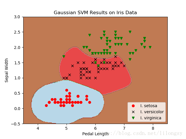
山鸢尾花(I.Setosa)非线性高斯SVM模型的多分类(三类)结果,其中gamma值为10
重点是改变SVM算法一次性优化三类SVM模型。模型参数b通过增加一个维度来计算三个模型。我们可以看到,使用TensorFlow内建功能可以轻松扩展算法到多类的相似算法。
以上就是本文的全部内容,希望对大家的学习有所帮助,也希望大家多多支持编程小技巧。
总结
以上是编程之家为你收集整理的用TensorFlow实现多类支持向量机的示例代码全部内容,希望文章能够帮你解决用TensorFlow实现多类支持向量机的示例代码所遇到的程序开发问题。
如果您也喜欢它,动动您的小指点个赞吧
 602392714
 清零编程群
清零编程群